Purpose Of This Blog

I recently implemented a couple of different architectures for LLMs, its quite nice to see how different each architecture is from each other and how they solve problems stemming from the same core architecture i.e , Drum roll … , Transformers!

One of the most interesting things that I stumbled across was RoPE (Rotary Positional Embeddings), so I decided to jump in on the rabbit hole of how everything worked for RoPE, from the paper, to a couple of videos and a I’d say about 15 different chats across Gemini, Grok and ChatGPT, I like to dig into how everything works, and naturally it takes time to learn everything, so I decided to consolidate almost everything behind RoPE in this blog, from the deficiencies in the original approaches, to the math, the intuition, the code. I guess time to dig into it.

Overview

I assume the audience who is reading this blog would have at least surface level knowledge of the following things:

What is a Transformer
What are Embeddings (Positional and Static)
What is Attention Mechanism

If not, I highly recommend going over through the following resources:

I’d still give a brief overview of the previous concepts, so it is a tad bit easier to follow along.

Embeddings

Embeddings are a way to represent words(tokens) in a continuous vector space. To make it simpler, an embedding is just a lookup table that maps a word(token) to a vector, these lookup maps are learned during the training process and are used to capture more semantic information about the words.

In a Transformer, the way information is processed is by passing the embeddings parallelly through the different layers of the transformer, this is done by passing the embeddings through a linear layer that projects the embeddings into a higher dimensional space.

Since transformers don’t have a sense of order, it is quite important to add/inject the position of the words being processed into the embeddings

This is where positional embeddings come into play, they are nothing but again a lookup table that maps a position to a vector.

In a nutshell the actual information, being passed to the transformer can be represented as the following equation:

\text{final\_embedding} = f_{\text{static}}(X) + f_{\text{positional}}(X)

Background of Positional Embeddings

Originally in the Transformer paper, the positional embeddings were added to the embeddings using a sine and cosine function. This was providing absolute positional information to the embeddings, and since the positional embeddings were sinusoidal, there was a linear relationship between different positions that was being captured. However, this had the following drawbacks:

They were not able to generalise to sequences longer than what was seen during training
They were not able to capture the relative position between two tokens

The equation for the same can be represented as the following:

\mathbf{q} = W_q(\mathbf{x} + PE(\mathbf{x}))

Where $\mathbf{q}$ is the query vector, $\mathbf{x}$ is the input vector, $W_q$ is the query projection matrix and $PE(\mathbf{x})$ is the positional embedding.

Another approach that was proposed was to take the relative distance between two tokens into account and add this as a learnable parameter, in this sense as a bias term to the attention score

\text{Attention}(Q, K, V) = \text{softmax}\left(\frac{QK^T + \mathbf{B}}{\sqrt{d_k}}\right)V

However, this approach also had drawbacks haha:

For each term that we were calculating the query vector, we had to calculate the bias term again and again, in a sense, adding a bias matrix to the computation, which if taken into account with KV Cache, would be a huge overhead in terms of memory and computation.

Rotary Positional Embeddings

So the ground was set in terms of what the inefficiencies were and how we could improve or make them better and that’s where RoPE comes into play.

Intuition

The intuition behind RoPE was derived from the following observations in the attention mechanism:

We need to capture the embedding information of the Key and The Queries
We need to capture the relative distance, in a sense, how does the position of the tokens influence the embedding information of the tokens

so in a sense, if all of this was to be summarised in a single equation which was inferred from the RoPE paper:

\langle f_q(x_m, m), f_k(k_n, n) \rangle = f(x_m, k_n, m-n)

the inner product i.e attention score between the query and the key should be a function of the query, the key and the relative distance between the two tokens

on a sidenote, math is so beautiful, isn’t it? but lets move on , I have to show the derivations as well :)

Pre Req Math

I so wanna show the derivations, but not without the proper math required, I read a lot of resources and GPTed through a lot of things, so I have to consolidate it over here

Rotation Matrix

A rotation matrix is special kind of matrix that is used to rotate a vector in a 2D space, it is a 2x2 matrix that is used to rotate a vector by a given angle.

The general form of a rotation matrix is the following:

\begin{bmatrix} \cos(\theta) & -\sin(\theta) \\ \sin(\theta) & \cos(\theta) \end{bmatrix}

One of the videos that I will recommend to understand the rotation matrix is the following: Rotation Matrix

This video is related in terms of Computer Vision, but the rotation matrix concept is the same and does a good job of explaining the concept.

Eulers Formula and Complex Numbers

A complex number is a number that is represented as a combination of a real part and an imaginary part. It is represented as $a + bi$ , where $a$ is the real part and $b$ is the imaginary part.

z = a + bi

Where $z$ is the complex number, $a$ is the real part and $b$ is the imaginary part.

A complex number can be represented as a point on the complex plane, where the real part is the x-axis and the imaginary part is the y-axis.

The magnitude of a complex number is given by the following formula:

|z| = \sqrt{a^2 + b^2}

now comes the best part

z = r e^{i\theta}

This is the polar form of a complex number, it is a way to represent a complex number in a more compact and intuitive way.

now comes the best part, Eulers Formula

e^{i\theta} = \cos(\theta) + i\sin(\theta)

this relates the exponential function to the trigonometric functions, it is a beautiful formula that relates the two and is used to represent complex numbers in a more compact and intuitive way.

Derivations of RoPE

So now that we have the pre req math out of the way, lets derive the RoPE stuff and how we can go about it.

There’s two ways to this, To keep this simple, I’ll assume the vectors that we are working with are 2D vectors and build up the derivations from the algebraic approach.

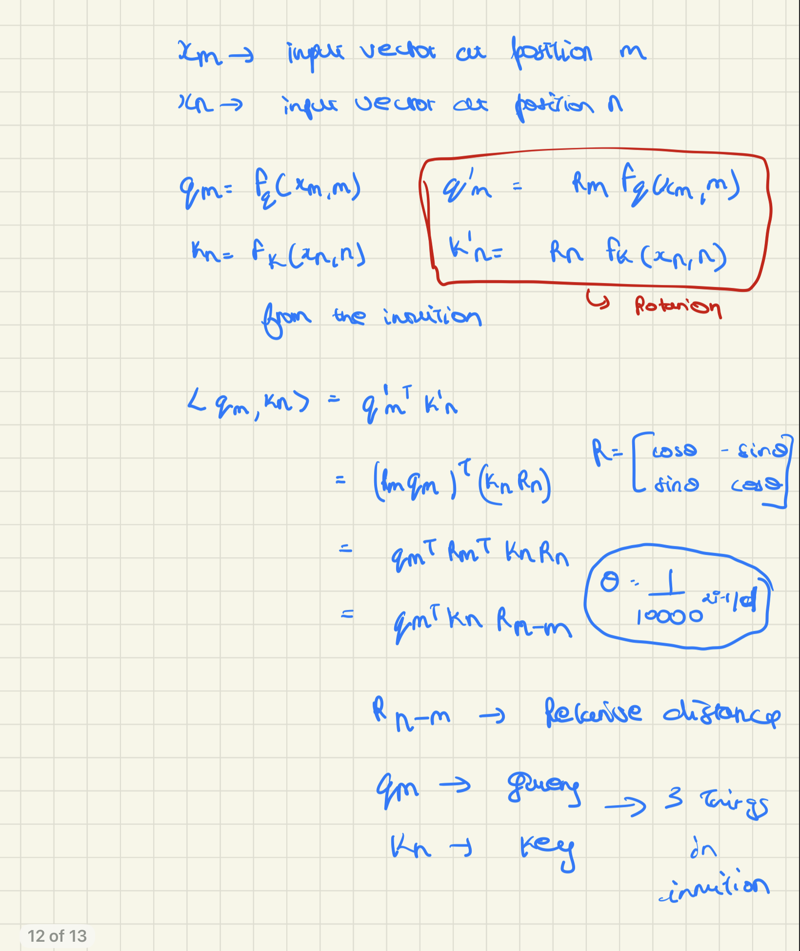
Algebraic Approach

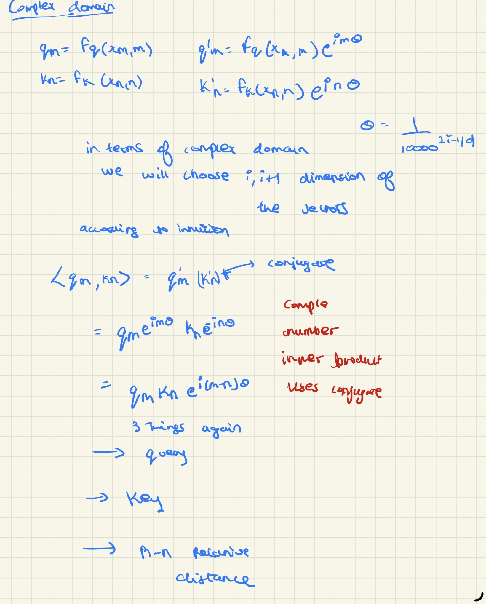
Complex Number Approach

Sparse Matrix For Higher Dimensions

So now that we have the derivations out of the way, lets talk about how we can extend this to higher dimensions.

In practice, our query and key vectors are not 2D—they’re typically much higher dimensional (e.g., 128, 256, 512, or even 4096 dimensions). To apply RoPE to these higher-dimensional vectors, we use a sparse block-diagonal matrix structure.

The Sparse Block-Diagonal Structure

For a $d$ -dimensional vector, we pair up dimensions and apply rotation matrices to each pair. Specifically:

Dimensions $(0, 1)$ get rotated together
Dimensions $(2, 3)$ get rotated together
Dimensions $(4, 5)$ get rotated together
And so on…

This creates a sparse block-diagonal matrix where each $2 \times 2$ block on the diagonal is a rotation matrix, and all off-diagonal elements are zero. This structure is computationally efficient because:

Most of the matrix is zeros (sparse), reducing memory and computation
Each rotation only affects a pair of dimensions, preserving the relative position encoding property
Matrix-vector multiplication becomes very efficient since we only need to process $2 \times 2$ blocks

Example: 6-Dimensional Vector

For a 6-dimensional query or key vector, the rotation matrix $\mathbf{R}_\theta$ would look like:

\mathbf{R}_\theta = \begin{bmatrix} \cos(\theta) & -\sin(\theta) & 0 & 0 & 0 & 0 \\ \sin(\theta) & \cos(\theta) & 0 & 0 & 0 & 0 \\ 0 & 0 & \cos(\theta) & -\sin(\theta) & 0 & 0 \\ 0 & 0 & \sin(\theta) & \cos(\theta) & 0 & 0 \\ 0 & 0 & 0 & 0 & \cos(\theta) & -\sin(\theta) \\ 0 & 0 & 0 & 0 & \sin(\theta) & \cos(\theta) \end{bmatrix}

Notice how:

The first $2 \times 2$ block rotates dimensions 0 and 1
The second $2 \times 2$ block rotates dimensions 2 and 3
The third $2 \times 2$ block rotates dimensions 4 and 5
All other entries are zero

In general, for a $d$ -dimensional vector with $d/2$ pairs, the rotation matrix has the form:

\mathbf{R}_\theta = \begin{bmatrix} \mathbf{R}_\theta^{(0,1)} & \mathbf{0} & \cdots & \mathbf{0} \\ \mathbf{0} & \mathbf{R}_\theta^{(2,3)} & \cdots & \mathbf{0} \\ \vdots & \vdots & \ddots & \vdots \\ \mathbf{0} & \mathbf{0} & \cdots & \mathbf{R}_\theta^{(d-2,d-1)} \end{bmatrix}

where each $\mathbf{R}_\theta^{(i,i+1)}$ is the $2 \times 2$ rotation matrix:

\mathbf{R}_\theta^{(i,i+1)} = \begin{bmatrix} \cos(\theta) & -\sin(\theta) \\ \sin(\theta) & \cos(\theta) \end{bmatrix}

Applying to Queries and Keys

When we apply RoPE to queries and keys at different positions $m$ and $n$ , we use different rotation angles:

Query at position $m$ : $\mathbf{q}_m = \mathbf{R}_{m\theta} \mathbf{q}$
Key at position $n$ : $\mathbf{k}_n = \mathbf{R}_{n\theta} \mathbf{k}$

The attention score becomes: $\mathbf{q}_m^T \mathbf{k}_n = (\mathbf{R}_{m\theta} \mathbf{q})^T (\mathbf{R}_{n\theta} \mathbf{k}) = \mathbf{q}^T \mathbf{R}_{m\theta}^T \mathbf{R}_{n\theta} \mathbf{k} = \mathbf{q}^T \mathbf{R}_{(m-n)\theta} \mathbf{k}$

This shows that the attention score depends only on the relative position $(m-n)$ , which is exactly what we want!

Implementation

So now that we have the math out of the way, lets implement RoPE in the codebase, I have taken this code out of Sebastian’s Blog on implementing Qwen 3, he is by far one of the most fluent person when it comes to LLMs, so I always refer to his resources

There’s 2 main functions:

one to calculate the RoPE embeddings.
one to apply the RoPE embeddings to the queries and keys.


def compute_rope(head_dim,seq_len,base_theta=10000):

    inv_freq = 1.0 / (base_theta ** (torch.arange(0, head_dim, 2) / head_dim)[:head_dim//2])
    m = torch.arange(seq_len,device=inv_freq.device)
    angles = m[:,None] * inv_freq[None,:]
    angles = torch.cat([angles,angles],dim=-1)
    cos = torch.cos(angles)
    sin = torch.sin(angles)
    return cos,sin

This function calculates the RoPE embeddings for a given head dimension, sequence length and base theta.

The base theta is a hyperparameter that is used to control the frequency of the RoPE embeddings.

The inv_freq is calculated using the base theta and the head dimension.

The m is calculated using the sequence length.

The angles are calculated using the m and the inv_freq.

The cos and sin are calculated using the angles, we need them to apply the RoPE embeddings


def apply_rope(x,cos,sin,offset):

    batch,num_heads,seq_len,head_dim = x.shape

    cos = cos[offset:offset+seq_len,:].unsqueeze(0).unsqueeze(0)
    sin = sin[offset:offset+seq_len,:].unsqueeze(0).unsqueeze(0)

    x1 = x[...,:head_dim//2]
    x2 = x[...,head_dim//2:]

    rotated_x = torch.cat([-x2,x1],dim=-1)

    rope_x = (x * cos) + (rotated_x * sin)

    return rope_x

This function applies the RoPE embeddings to the queries and keys.

The x is the input tensor, the cos and sin are the RoPE embeddings, the offset is the starting position of the RoPE embeddings.

The x1 and x2 are the even and odd dimensions of the input tensor.

The rotated_x is the rotated version of the x2.

The rope_x is the RoPE embeddings applied to the input tensor.

The offset is due to KV Cache logic, if you want to know more about it, I have a blog on it here

Conclusion

I hope this blog has helped you to understand the concept of RoPE and how it works, I have spent a whole lot of time understanding how this works, whats the math and the code (this wasn’t easy to find lol, I even toyed around with my own code and made something that worked, but couldn’t be used in a production codebase lol)

This still might not be perfect, but I have tried my best to explain it in a way that is easy to understand and please mind my handwriting in the derivations lol.

Rotary Positional Embeddings and its Math