Purpose Of This Blog

As part of me exploring different internal things about LLMs, this blog is about, if not the most, but one of the most important and misunderstood concepts in the field of LLMs, Normalization Techniques. I happen to stumble across this concept while reading through a couple of different resources, and I thought it would be a good idea to write about it, since it is such a fundamental concept in the field of LLMs.

The math behind normalization is quite simple, it’s not going to be like the math behind RoPE LOL, but it’s still quite interesting to see how it works and how it is used in the field of LLMs.

Math Concepts

For this blog, the three things that you need to know are (and might already know them from high school):

Mean

$\mu = \frac{1}{N} \sum_{i=1}^{N} x_i$
Variance

$\sigma^2 = \frac{1}{N} \sum_{i=1}^{N} (x_i - \mu)^2$
Standard Deviation

$\sigma = \sqrt{\sigma^2}$

Why Normalization is Needed

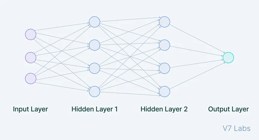
When we talk about neural networks, we have to visualise a lot of layers and the data passing through them, the following image is a good example of what a sample neural network layer looks like:

Neural Network Layer

There are two major processes that happen in a NN Layer

Forward Pass

In layman’s terms, the forward pass is the process of passing the data through each and every layer of the neural network once

Backward Pass or Backpropagation

In layman’s terms, this is the process of updating the weights of the neural network based on the loss between the predicted output and the actual output. This is done using the gradient descent algorithm.

Now forward pass is simple, and to be fair quite easy to get a grip on, but the real magic happens in the backward pass

In backpropagation, we calculate the gradient of each weight in the neural network with respect to the loss function. Mathematically speaking this is done using the chain rule, (I would love to talk about this, but this itself is a whole blog post and again I love to write about Math but that’s for another blog post)

Now during the backward pass, we update the weights based on the gradients calculated, but this paves the way for another problem

In a neural network the data coming as input for one layer is the output of the previous layer

So each layer adapts to the distribution of the data coming in, and this is where the problem lies, if the distribution of the data coming in is very different from the distribution of the data seen during previous steps, the model will not be able to learn effectively.

The layers are already adapting to the distribution but if due to the weight change, the distribution changes, the model will take longer to converge with more updates.

So we needed a way to find common grounds for the data coming in to the layers, and this is where normalization techniques come into play.

Batch Normalization

Batch Normalization is a technique that normalizes the data coming in to the layer by calculating the mean and variance of the data but across the batch rather than the entire feature space for a particular token

This was one of the most popular normalization techniques in the field of Neural Networks, and personally I have used it with CNNs

They aren’t used with Transformers, due to the following reasons:

Transformers are designed to process sequences of tokens, and batch normalization is not designed to handle sequences of varied length, on the other hand CNNs work so well with batch norm because they are designed to process data which is uniform in nature, IMAGES!!!
Another reason is that batch normalization maintains a running average and variance of the data across different batches, and when we go into training, we have distributed GPUs, so the running average and variance of the data across different GPUs would be different, and this would cause the model to not converge effectively.

Now lets look into how other techniques that are used in Transformers are different from batch normalization:

Layer Normalization

Layer Normalization is a technique that normalizes the data coming in to the layer by calculating the mean and variance of the data but across the feature space for a particular token

This was used in the original GPT-2 architecture and it was one of the most popular normalization techniques in the field of Transformers

the equation for layer normalization is as follows:

\mathbf{y} = \frac{\mathbf{x} - \mu}{\sqrt{\sigma^2 + \epsilon}} \cdot \gamma + \beta

Where $\mathbf{x}$ is the input data, $\mu$ is the mean, $\sigma$ is the standard deviation, $\gamma$ is the scale parameter and $\beta$ is the shift parameter, $\epsilon$ is a small constant to avoid division by zero

The normalization formula is pretty simple, but you might be wondering why we have two parameters, $\gamma$ and $\beta$ . After normalization, the data is centered around zero with unit variance, which can be too restrictive for the model to learn effectively. The learnable parameters $\gamma$ and $\beta$ allow the model to learn the optimal scale and shift for the normalized data, giving it the flexibility to adjust the normalization to what works best for learning. This way, if the model needs to undo some of the normalization or adjust it optimally, it can learn to do so through these parameters.

the code for the layer normalization is as follows:

class LayerNormalization(nn.Module):
    def __init__(self,emb_dim):
        super().__init__()
        self.scale = nn.Parameter(torch.ones(emb_dim))
        self.bias = nn.Parameter(torch.zeros(emb_dim))
        self.eps = 1e-6
    
    def forward(self,x):
        mean = torch.mean(x,dim=-1,keepdim=True)
        var = torch.var(x,dim=-1,keepdim=True)

        return ((x - mean) / torch.sqrt(var+self.eps)) * self.scale + self.bias

Now this proved to be quite effective in the field of Transformers, but researchers discovered another method that had similar results but was optimised

Root Mean Square Layer Normalization

Root Mean Square Layer Normalization is a technique that normalizes the data coming in to the layer by calculating the root mean square of the data

The research paper that introduces this technique argued that the normalization is a product of two different math techniques, one is shifting the data to the mean and the other is scaling the data to the standard deviation

The researchers found that most of the effect of normalization came through the effect of scaling and found that shifting the data had negligible returns.

the formula for RMS Layer Normalization is as follows:

\mathbf{y} = \frac{\mathbf{x}}{rms(\mathbf{x})} \cdot \gamma

rms(\mathbf{x}) = \sqrt{\frac{1}{N} \sum_{i=1}^{N} x_i^2}

the formula for RMS might look a bit daunting, but the idea to remember it is hidden in plain sight i.e SQUARE

ROOT
MEAN
SQUARE

which means, take the square of the input data, then take the mean of the squares, then take the square root of the mean and voila we get RMS

Parameter-Free RMSNorm

Interestingly, many modern transformer architectures have adopted a simplified version of RMSNorm that completely removes the learnable parameters. This parameter-free variant has gained significant popularity for several compelling reasons:

Why Remove Learnable Parameters?

The original RMSNorm research demonstrated that the primary benefit of normalization comes from dividing by the RMS value itself, not from the learnable affine transformation parameters. The researchers found that:

The core normalization effect comes from RMS scaling
Removing learnable parameters doesn’t negatively impact model performance
Training becomes more stable with the simpler normalization approach

Mathematical Simplification

Original RMSNorm with learnable parameters:

output = x * gamma / sqrt(mean(x²) + epsilon)

Parameter-free RMSNorm:

output = x / sqrt(mean(x²) + epsilon)

now the main code for the parameter-free RMSNorm is as follows:

class RMSNorm(nn.Module):
    
    def __init__(self,emb_dim,has_learnable_params:bool = True):
        super().__init__()
        self.scale = nn.Parameter(torch.ones(emb_dim))
        self.eps = 1e-6
        self.has_learnable_params = has_learnable_params
    
    def forward(self,x:torch.Tensor):
        rms = x.pow(2).mean(dim=-1,keepdim=True)
        norm_x = x * torch.rsqrt(rms+self.eps)

        if self.has_learnable_params:
            return norm_x * self.scale
        return norm_x

RMSNorm is optimised due to it only calculating one statistical measure i.e RMS, rather than calculating two i.e mean and variance, which believe it or not is a lot faster to compute and reduces computational overhead.

Conclusion

Well this blog is a pretty short and sweet version of what I usually write, I just enjoy writing about math and internals of LLMs, cause LLMs at the core represent a lot of deep math being applied practically and to the real world applications, and I think it’s a good idea to understand the math behind the scenes.

Since high school, I have always heard people mocking math and emphasising on statements like " Oh how is COS and SINE gonna help us in the real world?"

Well… when you look at LLMs, you see the world of math being illustrated beautifully, and statements like those become obsolete.

Anyways, I hope you enjoyed reading about this simple yet misunderstood concept in the field of LLMs.